Numbers Programmers Should Know About Hash
There is a hash table:
- It has
bbuckets. - It has
nkeys stored in it. - We assume that the hash function distributes keys uniformly.
- A bucket can contain more than 1 keys.
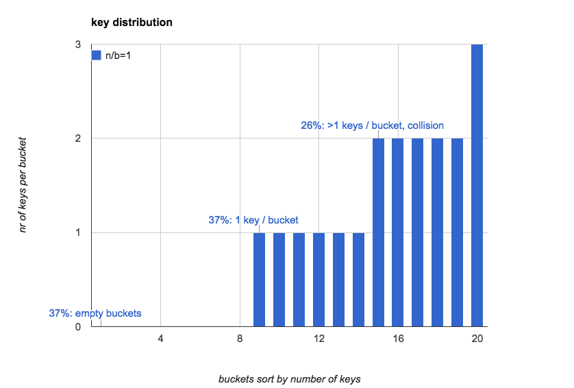
If n \(\approx\) b, the hash table would look like this:
- 37% buckets are empty.
- 37% buckets contain 1 key.
- 26% buckets contain more than 1 key, which means collision occurs.
The following chart created by program simulation shows distribution of 20 keys over 20 buckets.
Load Factor and Key Distribution
Let load factor \(\alpha\) be: \(\alpha = \frac{n}{b}\).
load factor defines almost everything in a hash table.
Load Factor <0.75
Normally in-memory hash table implementations keep load factor lower than
0.75.
This makes collision rate relatively low, thus looking up is very fast.
The lower the collision rate is, the less the time it takes to resolve collision,
since linear-probing is normally used and it is very sensitive to collision
rate.
In this case, there are about 47% buckets empty. And nearly half of these 47% will be used again by linear-probing.
As we can see from the first chart, when load factor is small, key
distribution is very uneven. What we need to know is how load factor affects
key distribution.
Increasing load factor would reduce the number of empty buckets and increase
the collision rate. It is monotonic but not linear, as the following table and
the picture shows:
Load factor, empty buckets, buckets having 1 key and buckets having more than 1 keys:
| load factor(n/b) | 0 | 1 | >1 |
|---|---|---|---|
| 0.5 | 61% | 30% | 9% |
| 0.75 | 47% | 35% | 17% |
| 1.0 | 37% | 37% | 26% |
| 2.0 | 14% | 27% | 59% |
| 5.0 | 01% | 03% | 96% |
| 10.0 | 00% | 00% | 100% |
![]()
0.75 has been chosen as upper limit of
load factornot only because of concerns of collision rate, but also because of the way linear-probing works. But that is ultimately irrelevant.
Tips
- It is impossible to use hash tables with low space overload and at the
same time, with low collision rate.
- The truth is that just enough buckets waste 37% space.
-
Use hash tables only for (in memory) small data sets.
-
High level languages like Java and Python have builtin hash tables that keep
load factorbelow 0.75. - Hash tables do NOT uniformly distribute small sets of keys over all buckets.
Load Factor >1.0
When load factor is greater than 1.0, linear-probing can not work any
more, since there are not enough buckets for all keys. chaining keys in a
single bucket with linked-list is a practical method to resolve collision.
linked-list works well only when load factor is not very large, since
linked-list operation has O(n) time complexity.
For very large load factor tree or similar data structure should be considered.
Load Factor >10.0
When load factor becomes very large, the probability that a bucket is empty
converges to 0. And the key distribution converges to the average.
The higher load factor is, the more uniformly keys are distributed
Let the average number of keys in each bucket be:
\[{avg} = \frac{n}{b}\]100% means a bucket contains exactly \({avg}\) keys.
The following charts show what distribution is like when load factor is 10,
100 and 1000:
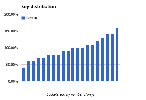
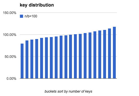
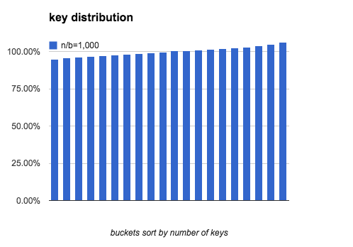
As load factor becomes higher, the gap between the most keys and the fewest
keys becomes smaller.
| load factor | (most-fewest)/most | fewest |
|---|---|---|
| 1 | 100.0% | 0 |
| 10 | 88.0% | 2 |
| 100 | 41.2% | 74 |
| 1,000 | 15.5% | 916 |
| 10,000 | 5.1% | 9735 |
| 100,000 | 1.6% | 99161 |
Calculation
Most of the numbers from above are produced by program simulations. From this chapter we are going to see what the distribution is in math.
Expected number of each kind of buckets:
0key: \(b e^{-\frac{n}{b}}\)1key: \(n e^{ - \frac{n}{b} }\)>1key: \(b - b e^{-\frac{n}{b}} - n e^{ - \frac{n}{b} }\)
Number of Empty Buckets
The chance a certain key is NOT in a certain bucket is: \(\frac{b-1}{b}\). Since: \(\lim_{b\to \infty} (1+\frac{1}{b})^b = e\). The probability of a certain bucket being empty is:
\[(\frac{b-1}{b})^n = ((1- \frac{1}b)^b)^{\frac{n}{b}} = e^{-\frac{n}{b}}\]Thus the total number of empty buckets is:
\[b e^{-\frac{n}{b}}\]Number of Buckets Having 1 Key
The probability of a bucket having exactly 1 key is:
\[{n \choose 1} ( \frac{1}{b} )^1 ( 1 - \frac{1}{b} )^{n-1} = \frac{n}{b} e^{-\frac{n}{b}}\]One of the
nkeys is in this bucket, and at the same time, no other key is in this bucket:
The the number of buckets having exactly 1 key is:
\[b\frac{n}{b} e^{-\frac{n}{b}} = n e^{ - \frac{n}{b} }\]Number of Buckets Having More Than One Key
\[b - b e^{-\frac{n}{b}} - n e^{ - \frac{n}{b} }\]Distribution Uniformity
Similarly, the probability of a bucket having exactly i keys is:
The probability distribution is binomial-distribution.
And we want to know how many keys there are in the bucket having the fewest keys and in the bucket having the most keys.
Approximation by Normal Distribution
When n and b are large, binomial-distribution can be approximated by
normal-distribution to estimate uniformity.
Let \(p = \frac{1}{b}\). The probability of a bucket having exactly i
keys is:
Where:
\[\mu = np \\ \sigma^2 = np(1-p) \\\]The probability that a bucket has less than x keys is:
Thus in this hash table, the total number of buckets having less than x keys is:
Choose x so that the total number of such buckets is 1. Then this only
bucket must be the one that has the fewest keys. So find x that satisfies:
With this x, the expected number of keys in this bucket is:
Since normal distribution is symmetric:
\[N_{max} + N_{min} = 2 \mu = 2 \frac{n}{b}\]Find x
Now what we need to do is to find x in order to find
\(N_{max}\) and \(\ N_{min}\).
The probability of a bucket that contains less than x keys is:
\(\Phi(x)\)
is cdf of standard normal distribution. When x - u is close to 0, it is
approximated by:
By iterating x backward from u to 0, we can find the solution to
Using this x we can find \(N_{min}\) and \(N_{max}\).
Simulations in Python
Several simulation programs used in this post are here: hash-simulation
Reference
Archive
- 15 Nov 2020 slimarray: gzip的压缩率, 即时访问
- 28 Oct 2020 200行代码实现基于paxos的kv存储
- 18 Oct 2020 后分布式时代: 多数派读写的'少数派'实现
- 20 Dec 2019 Art of Pull Requests(翻译)
- 21 Nov 2019 掐指算算: 你的CDN多花了几百万?
- 19 Nov 2019 一年的素描练习
- 30 Oct 2019 互联网中对象访问频率的91分布
- 09 Jan 2019 哄好面试官系列-1: 比较2个python dict(多级)是否相同
- 04 Nov 2018 存储中的文件合并策略优化
- 27 Sep 2018 软件工程是个面包机
- 26 Aug 2018 程序员必须知道的事情, 一般人我不告诉他
- 16 Aug 2018 cgexec 无法继承 LD_PRELOAD 环境变量
- 04 Aug 2018 mysql group replication实践记录: 步骤, 问题和注意事项
- 13 Feb 2018 枚举所有整勾股数
- 03 Feb 2018 ansible中的include, include_tasks 和 import_tasks 的差别
- 20 Nov 2017 python 并发subprocess.Popen的坑
- 05 Aug 2017 程序员必读: 摸清hash表的脾性
- 06 May 2017 python 进程内存增长问题, 解决方法和工具
- 01 Feb 2017 xp的分布式系统系列教程之: Erasure-Code: 工作原理, 数学解释, 实践和分析.
- 01 Feb 2017 xp的分布式系统系列教程之: Erasure-Code: 工作原理, 数学解释, 实践和分析.
- 11 Nov 2015 可靠分布式系统基础 Paxos 的直观解释
- 28 Jul 2015 socket关闭: close()和shutdown()的差异
- 17 May 2015 随手改变世界之 git-auto-squash
- 17 Feb 2015 Numbers Programmers Should Know About Hash
- 11 Feb 2015 Vim-tabbar: Simple, stupid and fast tab-bar for VIM
- 24 Jul 2014 1% 慢请求优化
- 31 Jan 2014 Some useful resources
- 31 Jan 2014 jobq.py -- Queue processing engine